PyTorch
Snippets of neural network definitions and other essential building blocks in PyTorch.
Boilerplate Structure of a PyTorch Program (Supervised Learning):
# PyTorch models can be deployed on a CPU or GPU
net = MyModel().to(device)

train_loader = torch.utils.data.DataLoader(...)
test_loader = torch.utils.data.DataLoader(...)

# Choosing an optimiser, eg. stochastic gradient descent, Adam, etc.
optimizer = torch.optim.SGD(net.parameters,...)

# Training is done in epochs
for epoch in range(1, epochs):
    train(params, net, device, train_loader, optimizer)
    if epoch % 10 == 0:
        test(params, net, device, test_loader)
Defining a Model
# Inherits from the torch.nn.Module class
class MyModel(torch.nn.Module):
    def __init__(self):
        super(MyModel, self).__init__()
        # The structure of the network is defined here

    def forward(self, input):
        # Run the input through the network and return the prediction
Defining a Custom Model
Consider the function $(x,y) \mapsto Ax\log (y) + By^2$,
class MyModel(torch.nn.Module):
    def __init__(self):
        super(MyModel, self).__init__()
        # The Parameter constructor needs to be given a torch tensor.
        # Here we're creating a tensor of size 1 and initialise it with a random Gaussian value
        # Since the aim is to tune this parameter, we set requires_grad=True
        self.A = nn.Parameter(torch.randn((1), requires_grad=True))
        self.B = nn.Parameter(torch.randn((1), requires_grad=True))
    def forward(self, input):
        output = self.A * input[:,0] * torch.log(input[:,1]) + self.B * input[:,1] * input[:,1]
Building a Neural Net from Individual Components:
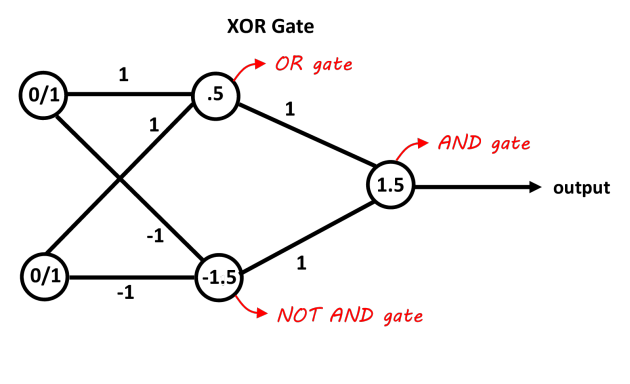
The following network would be suitable model for the XOR multi-layer perceptron.
class MyModel(torch.nn.Module):
    def __init__(self):
        super(MyModel, self).__init__()
        # From an input layer with 2 nodes to a hidden layer with 2 nodes
        self.in_to_hid  = torch.nn.Linear(2, 2)
        # From a hidden layer with 2 nodes to an output layer with 1 node
        self.hid_to_out = torch.nn.Linear(2, 1)

    def forward(self, input):
        # Takes the input vector and multiplies it with the weight matrix from input layer -> hidden layer
        hid_sum = self.in_to_hid(input)

        # Apply tanh on each component of the hidden layer's output
        hidden  = torch.tanh(hid_sum)

        # Matrix multiplication of hidden layer output with the weights going into the output layer
        out_sum = self.hid_to_out(hidden)

        # Applying the sigmoid function on the final output
        output  = torch.sigmoid(out_sum)
        return output
Defining a Sequential Network:
Modules are added in the order that they are passed into the $\texttt{Sequential}$ constructor.
class MyModel(torch.nn.Module):
    def __init__(self, num_input, num_hidden, num_out):
        super(MyModel, self).__init__()
        self.main = nn.Sequential(
            nn.Linear(num_input, num_hidden),
            nn.Tanh(),
            nn.Linear(num_hidden, num_out),
            nn.Sigmoid()
        )
    def forward(self, input):
        output = self.main(input)
        return output
Sequential Components:
Neural network layers:
- $\texttt{nn.Linear()}$ — for linear layers
- $\texttt{nn.Conv2d()}$ — for 2D convolutional layers
Intermediate operators — these are applied prior to the activation function
- $\texttt{nn.Dropout()}$
- $\texttt{nn.BatchNorm()}$
Activation functions:
- $\texttt{nn.Tanh()}$
- $\texttt{nn.Sigmoid()}$
- $\texttt{nn.ReLU()}$
Working With Data:
The following snippet declares the input dataset for the XOR network and the expected output predictions.
import torch.utils.data

input    = torch.Tensor([0, 0],
                        [0, 1],
                        [1, 0],
                        [1, 1])
expected = torch.Tensor([0],
                        [1],
                        [1],
                        [0])

# TensorDataset forms the training dataset from the input samples and corresponding target outputs
xdata        = torch.utils.data.TensorDataset(input, expected)
train_loader = torch.utils.data.DataLoader(xdata, batch_size=4)
Batch size:
Batch size is a hyperparameter of gradient descent. The $\texttt{batch_size}$ defines the number of input datapoints to be propagated through the network, after which, the network's weights are updated.
Eg. specifying a batch size of 100 will use the first 100 datapoints from the input dataset to train the network for the first training iteration. For the next iteration, it takes the next 100 datapoints from the input dataset to train the network, and so on.
Training in mini-batches:
- Requires less memory. You can't fit a massive dataset in memory all at once
- Weights are learned more quickly since we are making updates after each batch is completed, as opposed to making 1 single update after the entire input dataset has been propagated through
- Becomes less accurate the smaller the batch
Epoch and Iterations:
An epoch is one complete iteration through the entire dataset, forward and backward through the network.
An iteration is the number of batches in 1 epoch.
Since gradient descent is an iterative process, making further epochs will converge the weights closer to 0% error. Only running one epoch usually leads to underfitting. Running too many epochs will usually lead to overfitting. The number of epochs depends on the diversity of the training dataset's samples.
import torchvision.datasets as dsets

mnist    = dsets.MNIST(...)       # Handwritten digits dataset
cifarset = dsets.CIFAR10(...)     # Animal and vehicle images dataset
celebset = dsets.CelebA(...)      # Celebrity pictures dataset
Choosing an Optimiser:
Constructing optimiser object in PyTorch:
net = MyModel.to(device)
...

# Stochastic gradient descent
optimiser = torch.optim.SGD(
    net.parameters(),
    lr=0.01,
    momentum=0.9,
    weight_decay=0.0001
)

# Adaptive moment estimation
optimiser = torch.optim.Adam(
    net.parameters(),
    eps=0.000001,
    lr=0.01,
    betas=(0.5, 0.999),
    weight_decay=0.0001
)
Training the Network:
A high-level structure for neural network training:
def train(args, net, device, train_loader, optimiser):
    for batch_index, (data, target) in enumerate(train_loader):
        optimiser.zero_grad()   # Zero the gradients
        output = net(data)      # Get prediction
        loss = ...              # Compute loss function
        loss.backward()         # Update gradients (backpropagate)
        optimiser.step()        # Update the weights
Loss Functions:
import torch.nn.functional as F

loss = torch.sum((output - expected) ** 2)       # Mean squared error

# Predefined loss functions
loss = F.nll_loss(output, expected)              # Negative log likelihood
loss = F.binary_cross_entropy(output, expected)  # Cross entropy (for a 2-class classification)
loss = F.softmax(output, dim=1)                  # Softmax
loss = F.log_softmax(output, dim=1)              # Log softmax
Testing the Network
def test(args, model, device, test_loader):
    # Suppress the update of gradients since we're meant
    # to leave the network unchanged in testing
    with torch.no_grad():
        # Toggles batch norm and dropout since these are for training purposes
        net.eval()

        test_loss = 0
        for data, target in test_loader:
            output = model(data)
            test_loss += ...
        print(test_loss)

        # Toggle batch norm and dropout after the testing is done
        net.train()
Computational Graph:
Controlling the Computational Graph:
"""
    If we need to block gradients from being backpropagated through
    a certain variable, A, we can exclude it from the computational
    graph with the detach method:
"""
A.detach()
"""
    loss.backward() discards the computational graph after computing
    the gradients. To keep the computational graph, set retain_graph=True
"""
loss.backward(retain_graph=True)
Tensors Theory:
Tensor — a rank-$n$ tensor in $m$-dimensions is a mathematical object with $n$ indices and $m^n$ components and obeys certain transformation rules.
- "Tensor" comes "to stretch" in Latin.
- A vector is a tensor
Continuum Mechanics:
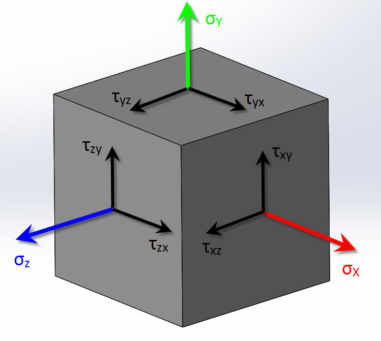
In continuum mechanics, stress is a physical quantity that expresses the internal forces that neighbouring particles of a continuous material exert on each other.
Consider a cube in 3D space. It can be 'stretched' in 3 separate dimensions and 'sheared' in 6 directions:
|
|
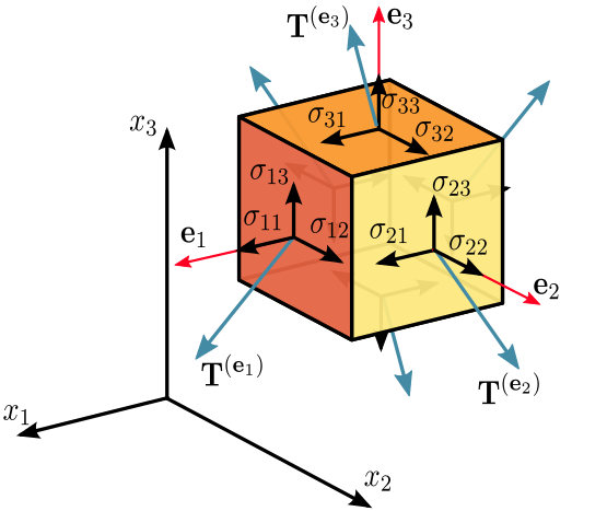
These 9 different stresses that can be applied to the cube are organised into a stress tensor like this: $ \begin{pmatrix} \sigma_{11} & \sigma_{12} & \sigma_{13} \\ \sigma_{21} & \sigma_{22} & \sigma_{23} \\ \sigma_{31} & \sigma_{32} & \sigma_{33} \\ \end{pmatrix} $. Each row and column correspond to a physical dimension (x, y and z).
*Rank* can be thought of as the amount of information you need to find a specific component. Formally, rank is the number of basis vectors required to fully specify a component of the tensor.
For example, since we can identify any $\sigma_{ij}$ by specifying the row and the column, we say that this tensor is rank-$2$ and $3$-dimension. Note that the number of components is given by $dim^{rank}=3^2=9$.
![]()
In general, we just use index notation instead of matrix notation to specify tensors, since matrix notation breaks beyond rank-$2$.
Note that a rank-$2$ tensor is not the same as a matrix. Fundamentally, a matrix is just a data structure for numbers. A tensor, on the other hand, is a data structure that obeys certain transformation rules.
Tensors have a deeper physical significance.
Transformation Rules:
- A tensor is invariant under a change in the coordinate system. During a change to the coordinate system, the components change according to a special set of equations, but the vector itself has not been affected. Eg. think of a displacement vector between two objects in 3D space — its components will certainly change if the coordinate system is rotated, displaced, etc., but the actual displacement vector itself preserves its physical meaning.
PyTorch Cookbook:
Dependencies:
import torch
import numpy as np
Tensors:
Tensors are multi-dimensional arrays with support for autograd operations like backward(). Tensors in PyTorch are similar to tensors in NumPy, except that they can be used on a GPU.
Creating Tensors:
- $\texttt{torch.rand(shape)}$ — returns a tensor with random values drawn from a uniform distribution on interval $[0, 1)$
- $\texttt{torch.zeros(shape)}$ — returns a tensor where all components are initialised with zeroes
- $\texttt{torch.tensor(data)}$ — creates a tensor from the supplied data list/array
Tensor Properties:
Tensors have the following methods:
- $\texttt{size()}$ — returns a tuple-like object containing the tensor's shape
- $\texttt{transpose(dim0, dim1)}$ — returns a transposed tensor
- Eg.
x.transpose(0, 1)transposes a 2D tensor
- Eg.
- $\texttt{reshape(shape)}$ — returns a reshaped tensor, containing the same data
x = torch.rand((2, 3))
print("===== Original tensor =====")
print(x)
print("Size: {}".format(x.size()))

x = x.transpose(0, 1)
print("===== Transpose =====")
print(x)

print("===== Reshape ====")
x = x.reshape((1, 6))
print(x)
Tensor operations:
The elementwise math operators +, -, *, / can be used on any two size-compatible tensors.
x = torch.tensor([1.0, 2.0, 3.0])
y = torch.tensor([4.0, 5.0, 6.0])
print("x = {}".format(x))
print("y = {}".format(y))

print("===== Operations =====")
print("x + y = {}".format(x + y))
print("x - y = {}".format(x - y))
print("x * y = {}".format(x * y))
print("x / y = {}".format(x / y))
Converting between torch tensor and numpy array:
import numpy as np

print("===== torch.Tensor to numpy.ndarray =====")
x = torch.tensor([1, 2, 3])
print("Torch tensor: {}".format(x))
x = x.numpy()
print("Numpy array:  {}".format(x))

print("===== numpy.ndarray to torch.Tensor =====")
x = np.array([1, 2, 3])
print("Numpy array:  {}".format(x))
x = torch.from_numpy(x)
print("Torch tensor: {}".format(x))
CUDA Tensors:
# The following this cell is only run if CUDA is available
# We will use `torch.device` objects to move tensors in and out of GPU
if torch.cuda.is_available():
    device = torch.device("cuda")          # a CUDA device object
    y = torch.rand((1, 3), device=device)  # directly create a tensor on GPU
    x = x.to(device)                       # or just use strings ``.to("cuda")``
    z = x + y
    print(z)
    print(z.to("cpu", torch.double))       # `.to` can also change dtype together!
Autograd — Automatic Differentiation:
The autograd package provides automatic differentiation for all operations on Tensors.
- Enabling tracking:
- Setting
requires_grad=Trueon a new tensor tracks all the computation done on it. Once the computations are done, you can call.backward()to have all the gradients computed automatically.
- Setting
- Disabling tracking:
.detach()method prevents computation tracking- Wrapping the code block in
with torch.no_grad()blocks tracking for everything within the block. Useful for when we're testing the model rather than training
Computation tracking example:
x = torch.ones(2, 2, requires_grad=True)
print("x = {}".format(x))

y = x + 2
print("y = {}".format(y))
print("y.grad_fn = {}".format(y.grad_fn))   # y was created as a result of an operation on x, so it has a grad_fn

z = y * y * 3
print("z = {}".format(z))
print("z.grad_fn = {}".format(z.grad_fn))

theta = z.mean()
print("Theta of z = {}".format(theta))
print("Theta.grad_fn = {}".format(theta.grad_fn))

# Doing backpropagation:  (note that calling backward() is only valid on a scalar)
theta.backward()

print("dθ/dx = {}".format(x.grad))
`Torch.nn`
nn.Module — base class for all neural network modules. Convenient for encapsulating parameters, keep track of state and has helpers for moving them to the GPU
parameters()— returns an iterator containing the network's parameterszero_grad()— zeroes the gradient buffers of all parameters. It's necessary to zero the gradients prior to backpropagation because PyTorch accumulates gradients on subsequent backward passes by default
Loss Functions:
There are several different error functions available in the nn package. They all take in an $\texttt{(prediction, target)}$ pair and give back a value that indicates the magnitude of prediction error
MSELoss— mean squared errorCrossEntropyLoss— cross entropy error
Optimisers (from torch.optim):
SGD(net.parameters(), lr, momentum)Adam([var, var2], lr)
Optimiser methods:
zero_grad()step()— updates the network parameters. Called once the gradients have been computed bybackward()
Building Blocks:
Linear(in_size, out_size)— applies linear transformation: $y=xA^T+b$Conv2d(in_channels, out_channels, kernel_size, stride, padding)— a 2D convolutional layerMaxPool2d()
PyTorch Example Models:
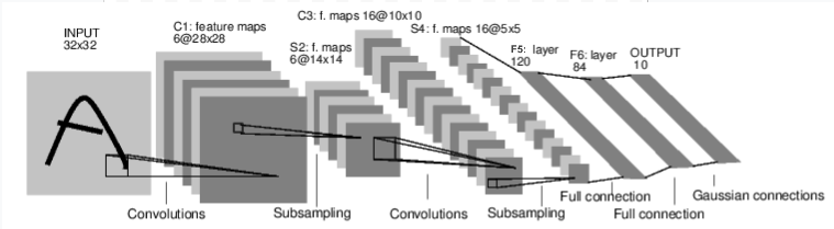
Handwritten Digits Classifier:
Below is a network that classifies handwritten digits.
import torch
import torch.nn as nn
import torch.nn.functional as F


class Net(nn.Module):

    def __init__(self):
        super(Net, self).__init__()

        # Convolutional layers
        self.conv1 = nn.Conv2d(1, 6, 3)  # 1 input image channel, 6 output channels, 3x3 convolution kernel
        self.conv2 = nn.Conv2d(6, 16, 3) # 6 input channels, 16 output channels, 3x3 kernels

        # Fully connected layers
        self.fc1 = nn.Linear(16 * 6 * 6, 120)  # 6*6 from image dimension
        self.fc2 = nn.Linear(120, 84)
        self.fc3 = nn.Linear(84, 10)

    # Note: the backward() function is automatically defined by autograd
    def forward(self, x):
        x = F.max_pool2d(F.relu(self.conv1(x)), (2, 2)) # Max pooling over a (2, 2) window on conv1
        x = F.max_pool2d(F.relu(self.conv2(x)), 2)      # Max pooling over a (2, 2) window on conv2
        x = x.view(-1, self.num_flat_features(x))       # Flattening(?)
        x = F.relu(self.fc1(x))
        x = F.relu(self.fc2(x))
        x = self.fc3(x)
        return x

    def num_flat_features(self, x):
        size = x.size()[1:]  # all dimensions except the batch dimension
        num_features = 1
        for s in size:
            num_features *= s
        return num_features


net = Net()
print(net)

# Network parameters are accessible under net.parameters()
print("Network parameters")
params = list(net.parameters())
for each_layer in net.parameters():
    print("    {}".format(each_layer.size()))
Predicting:
# Making a prediction, zeroing the gradients, then backpropagating:

input = torch.randn(1, 1, 32, 32)
out = net(input)
print("Output layer: {}".format(out))

net.zero_grad()   # Need to zero the gradients prior to backpropagation
out.backward(torch.randn(1, 10))
Computing Loss:
output = net(input)
target = torch.randn(10) # a dummy target, for example
target = target.view(1, -1) # Flatten it to the same shape as output
criterion = nn.MSELoss()
loss = criterion(output, target)
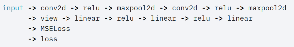
print(loss)
This is the sequence of computations in a forward pass:
Backpropagation:
Now, calling loss.backward(), the whole computational graph is differentiated.
net.zero_grad()     # zeroes the gradient buffers of all parameters

print('=== conv1.bias.grad before backward() ===')
print(net.conv1.bias.grad)

loss.backward()

print('=== conv1.bias.grad after backward() ===')
print(net.conv1.bias.grad)
Using optimisers:
All that's left to do at this point is to update the weights using an optimiser.
import torch.optim as optim

optimiser = optim.SGD(net.parameters(), lr=0.01)

# This goes in the training loop:
optimiser.zero_grad()
output = net(input)
loss = criterion(output, target)
loss.backward()
optimiser.step()      # step() proceeds with the update