Neural Network Learning and Backpropagation:
Ockham's Razor:
Ockham's razor is a problem-solving principle that asserts that "the most likely hypothesis is the simplest one consistent with the data"
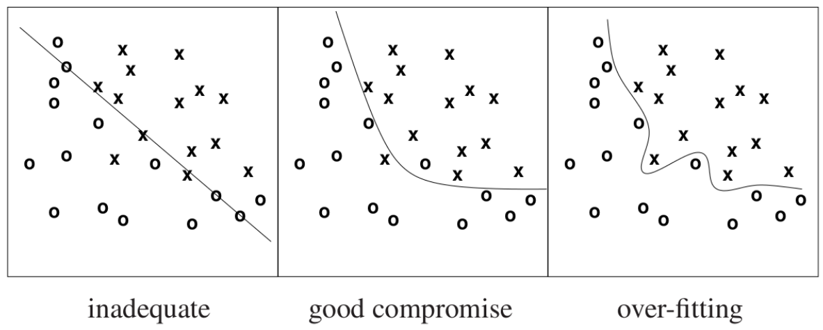
Overfitting is when the learning model is too fine-tuned to the noise rather than the true signal. In the third panel above, the network has learned a decision boundary that doesn't generalise to the true pattern presented by the dataset.
Training Neural Networks:
In the context of neural networks, learning is the process of adjusting a network's weights to achieve a configuration that minimises the error function.
Error Functions:
An example error function, also called loss function, that can be used to quantify the incorrectness of a network's prediction is the mean squared error function.
Mean squared error — the sum of the squared difference between the network's predicted value $z_i$ and the expected value $t_i$ for all $i$ neurons in the output layer: $$ E(z_i, t_i)=\frac{1}{2}\sum_{i} (z_i-t_i)^2. \tag{1} $$ Note the $\frac{1}{2}$ is chosen so that the coefficient is conveniently canceled when we differentiate this error function with respect to a network weight.
Cross-entropy loss — ... for all $i$ neurons in the output layer: $$ E(z_i, t_i)=-\sum_{i}t_i\log{(z_i)}. \tag{2} $$ Cross-entropy is a good error function for measuring the 'distance' between the vector of the output layer's predicted probabilities for each class and the expected label vector, which is 1-hot encoded.
- Binary cross-entropy loss — a variation on regular cross-entropy loss
- Categorical cross-entropy loss — also called softmax loss. It is just softmax followed by a cross-entropy loss
The cost function computes the average of the loss function values across the entire training set: $\frac{1}{m}\sum_{i=1}^m E(z^{(i)}, t^{(i)})$, where $m$ is the total number of training examples and $z^{(i)}$ and $t^{(i)}$ are the prediction and target value for the $i^{\text{th}}$ training sample respectively.
Differentiable Activation Functions:
A requirement for backpropagation in neural networks is a differentiable activation function, since backpropagation uses gradient descent to adjust weights.
The Heaviside step function's derivative has a value of $0$ everywhere, so gradient descent can't make progress in updating the weights. One very important transition beyond the perceptron model is the introduction of continuous activation functions.
Alternative differentiable activation functions:
- Logistic sigmoid: $\sigma(s) =\frac{1}{1+e^{-s}}$
- Output values range: $[0, 1]$
- In statistics, logistic regression is used to model the probability of a binary event (eg. alive/dead, cat/non-cat, etc.). Like all regression analyses, logistic regression is a form of predictive analysis
- Hyperbolic tan: $\texttt{tanh}(s)=\frac{e^s-e^{-s}}{e^s+e^{-s}}=2(\frac{1}{1+e^{-s}}) - 1=2\sigma(s)-1$
- Output values range: $[-1, 1]$
- $\texttt{tanh}$ is just the logistic sigmoid function doubled and then shifted down 1 unit vertically
- Rectified linear unit — $\texttt{ReLU}(s) = \begin{cases} x, & s > 0,\\ 0, & s \leq 0. \end{cases}$
Gradient Descent:
Gradient descent is an optimiser algorithm that neural networks can use to update individual weights. It works by repeatedly application of the following update rule: $$ w_{jk} := w_{jk} - \eta \frac{\partial E}{\partial w_{jk}} \tag{3} $$
where the term $\frac{\partial E}{\partial w_{jk}}$ is computed through backpropagation. The term $\frac{\partial E}{\partial w_{jk}}$ can be thought of as a measurement of how much the error function $E$ changes when we make a very small change to $w_{jk}$.
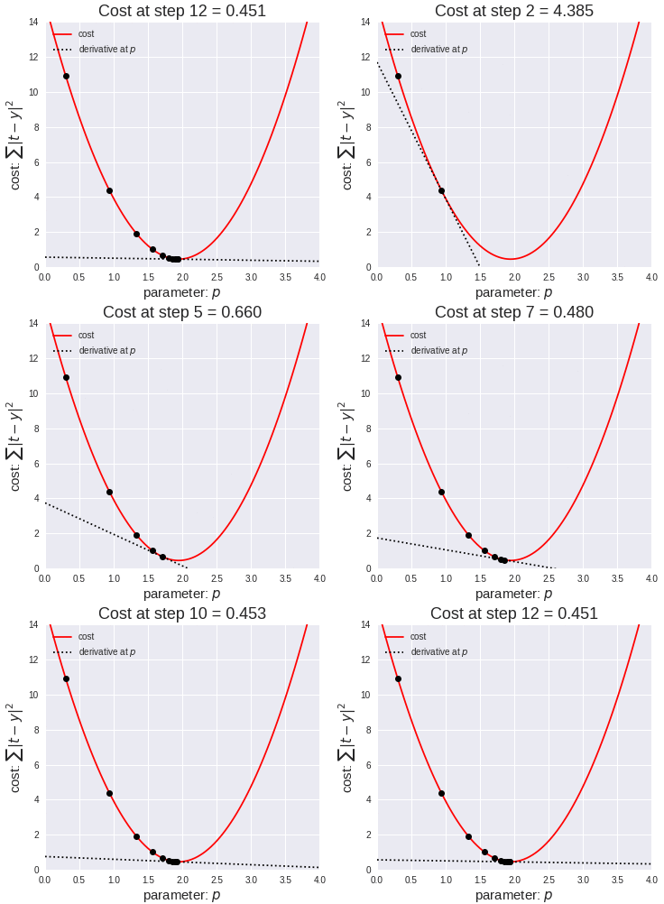
With every iteration of $(3)$, the weight $w_{jk}$ takes a 'step' downhill the error landscape. Eventually, the weight $w_{jk}$ will settle on a value that is a local minimum.
A very large learning rate could cause the updated weight value to overstep the local minimum and spiral up the error landscape. A very low learning rate means the network converges on optimal weight values slower.
|
We want all weights to take on the global minimum value, but depending on the learning rate and what value the weight initially starts with, gradient descent may cause the weight to settle on a value corresponding to a suboptimal local minimum instead. 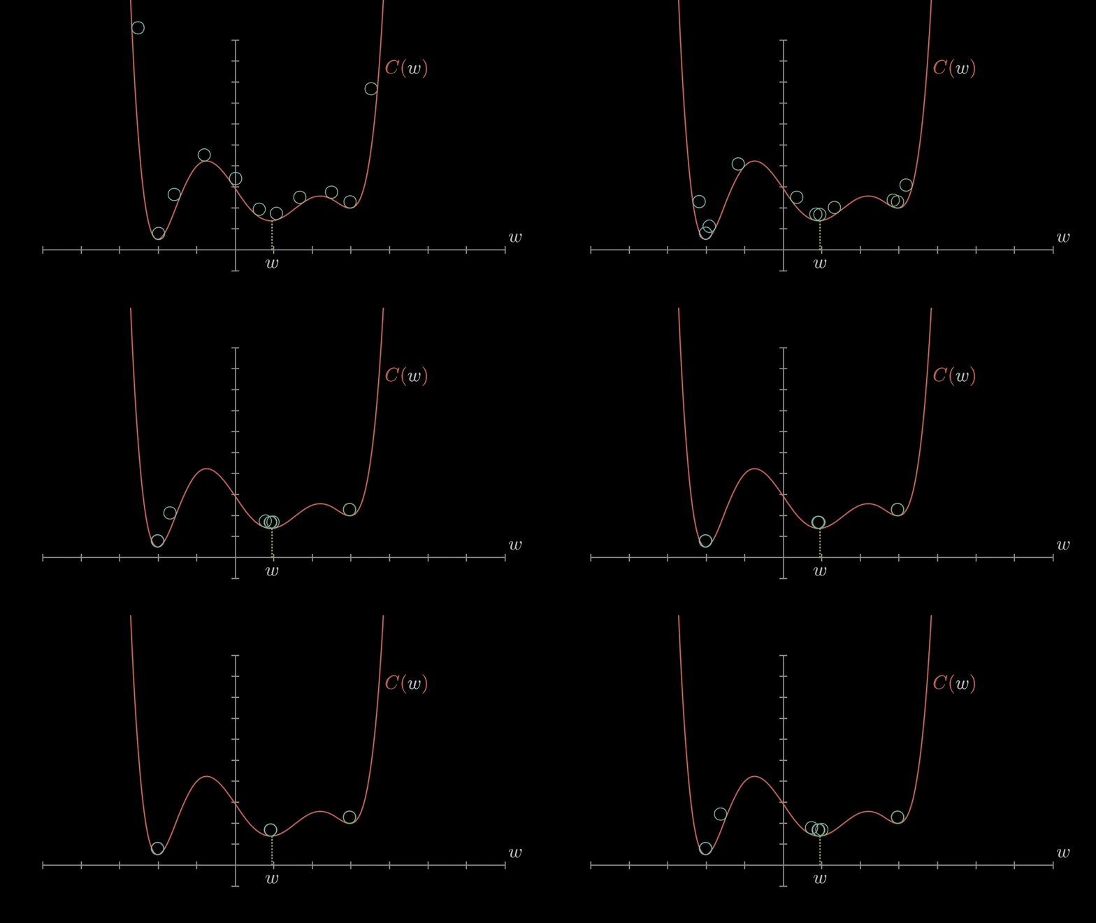
|
There are variations on gradient descent which introduce concepts like momentum and acceleration.
There also exists many other optimisers such as adagrad, adam, rms-prop, Nesterov accelerated gradient, etc.
Momentum:
With gradient descent + momentum, we're introducing a momentum factor, $\delta w$, which retains a proportion of the previously computed gradient $\frac{\partial E}{\partial w}$ for use in the current weight update:
Backpropagation
Backpropagation is an algorithm for computing the derivative of the error function $E$ with respect to individual network weights $w_{ij}$. It is just the systematic application of chain rule starting from the output layer, and passing intermediate results backwards so that earlier derivatives that depend on derivatives from later layers can be computed.
Backpropagation From First Principles:
|
Example neural network 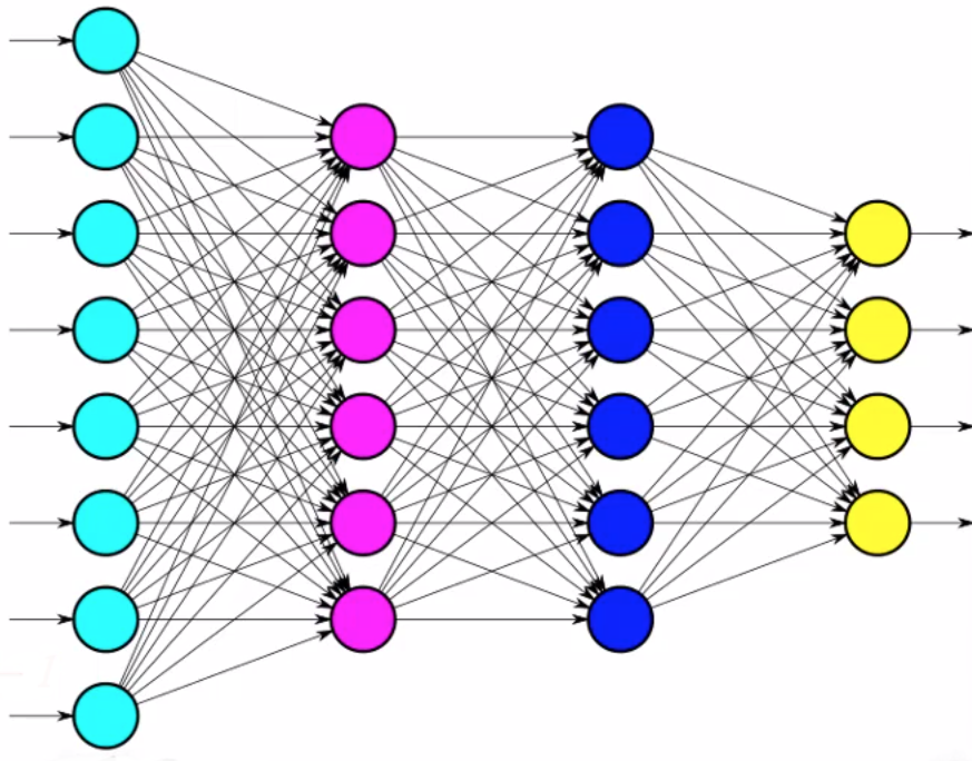
|
Weight component $w_{jk}^{(l)}$ 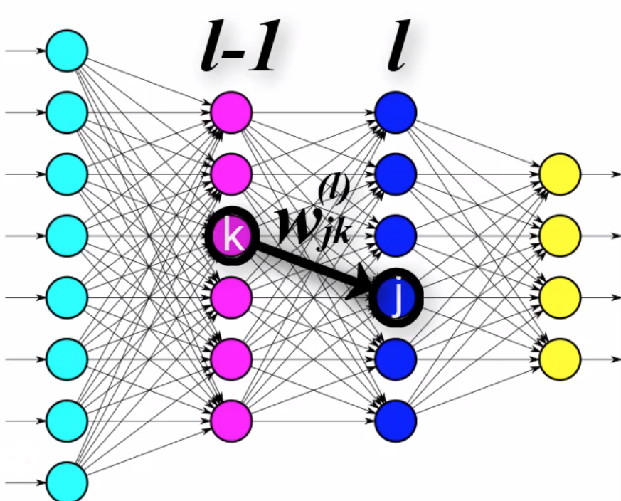
|
Weight vector $w_{j}^{(l)}$ 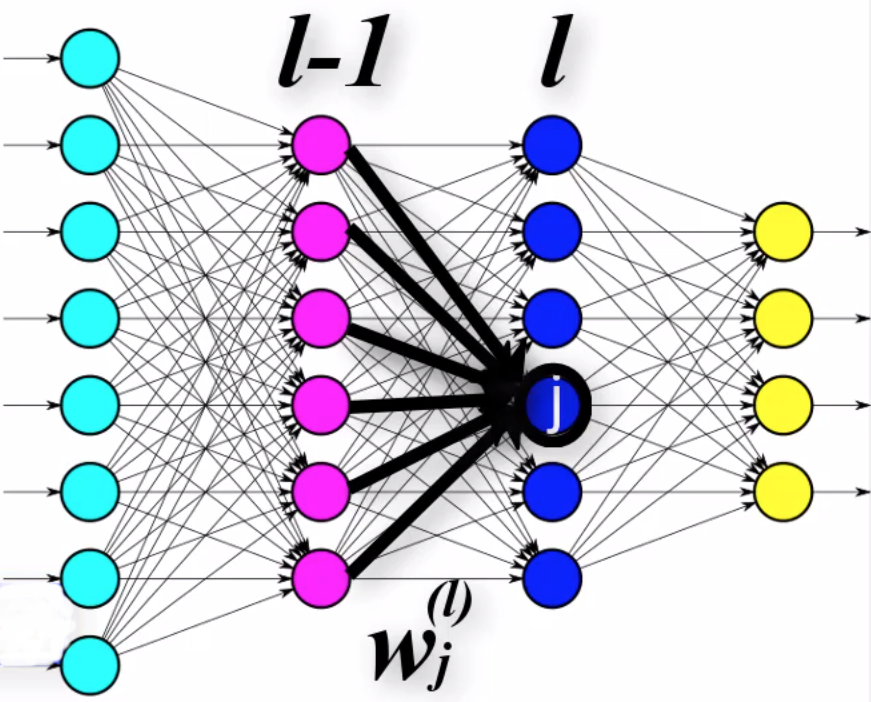
|
Mathematical Notation:
- $L$ — number of layers in the network
- $l$ — indexing variable for layers $1, 2, \ldots, L-1, L$
- $j$ — indexing variable for node $j$ in layer $l$
- $k$ — indexing variable for node $k$ in layer $l-1$
- $n$ — the number of nodes in layer $l$
- $m$ — the number of nodes in layer $l-1$
- $y_j$ — the expected value of output node $j$ in the output layer
- $E$ — error function for a single input
- $w_{jk}^{(l)}$ — the specific weight that connects to node $j$ in layer $l$ from node $k$ in layer $l-1$
- $w_{j}^{(l)}$ — the vector of all weights from layer $l-1$ towards node $j$ in layer $l$
- $z_j^{(l)}$ — the weighted sum of inputs into node $j$ at layer $l$
- $g^{(l)}$ — the activation function applied on the nodes of layer $l$
- $a_j^{(l)}$ — the activation value outputted by node $j$ at layer $l$
Error Function as a Composition of Functions:
Suppose we're using the mean squared error function, $(1)$, as our network's error function: $$E=\frac{1}{2}\sum_{j=0}^{n-1} (a_{j}^{(L)}-y_j)^2.$$
The activation value $a_j^{(L)}$ is given by: $$ \begin{align} a_j^{(L)}&=g^{(L)}\big( z_j^{(L)}\big) \\ &= g^{(L)} \big( \sum_{k=0}^{m-1} w_{jk}^{(L)} \cdot a_k^{(L-1)} \big). \end{align} $$
Now, the error function can be expressed as: $$ E=\frac{1}{2}\sum_{j=0}^{n-1} \Bigg( \underbrace{g^{(L)} \big( \sum_{k=0}^{m-1} w_{jk}^{(L)} \cdot a_k^{(L-1)} \big)}_{a_j^{(L)}} -y_j\Bigg)^2. \tag{a} $$
The main point is that we recognise that $(a)$ is just a function composition: $$ \begin{align} E&=\sum_{j=0}^{n-1} E(a_{j}^{(L)}), \tag{$E$ is a function of the activation value} \\ &=\sum_{j=0}^{n-1} E(a_{j}(z_{j}^{(L)})), \tag{$a$ is a function of the weighted sum} \\ &=\sum_{j=0}^{n-1} E(a_{j}(z_{j}^{(L)}(w_j^{(L)}))). \tag{$z$ is a function of the weights} \\ \end{align} $$
Backpropagation Algorithm Derivation:
Gradient descent requires that we know what the value of $\frac{\partial E}{\partial w_{jk}^{(l)}}$ is for all individual weight parameters $w_{jk}^{(l)}$ in the network. Let's focus on how to calculate the gradient of the error function with respect to one specific weight $w_{12}^{(L)}$, which is $\frac{\partial E}{\partial w_{12}^{(L)}}$, for now.
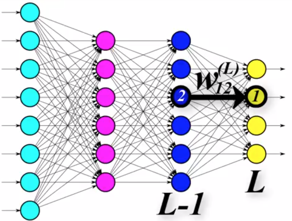
From the previous observation that the error function is a function composition of the activation function and the weighted sum function, we can use the chain rule to obtain $\frac{\partial E}{\partial w_{12}^{(L)}}$: $$ \frac{\partial E}{\partial w_{12}^{(L)}} = \underbrace{\frac{\partial E}{\partial a_{1}^{(L)}}}_{\text{term 1}} \cdot \underbrace{\frac{\partial a_{1}^{(L)}}{\partial z_{1}^{(L)}}}_{\text{term 2}} \cdot \underbrace{\frac{\partial z_{1}^{(L)}}{\partial w_{12}^{(L)}}}_{\text{term 3}}. \tag{b} $$
Computing Term 1:
We're using the mean squared error, so we have $$ E=\frac{1}{2}\sum_{j=0}^{n-1} (a_{j}^{(L)}-y_j)^2. $$ Calculating the derivative of $E$ with respect to $a_1^{(L)}$, $$ \begin{align} \frac{\partial E}{\partial a_1^{(L)}}&=\frac{\partial}{\partial a_1^{(L)}} \Bigg(\frac{1}{2}\sum_{j=0}^{n-1} (a_{j}^{(L)}-y_j)^2 \Bigg),\\ &= \frac{\partial}{\partial a_1^{(L)}} \Bigg(\frac{1}{2} \Big( (a_{0}^{(L)}-y_0)^2 + (a_{1}^{(L)}-y_1)^2 + \ldots + (a_{n-1}^{(L)}-y_{n-1})^2 \Big) \Bigg), \\ &= \frac{\partial}{\partial a_1^{(L)}} \Bigg(\frac{1}{2} \Big( a_{1}^{(L)}-y_1 \Big)^2 \Bigg), \\ &= a_{1}^{(L)}-y_1. \\ \end{align} $$
Computing Term 2:
The activation function is given by $$ a_{1}^{(L)} = g^{(L)}\big(z_1^{(L)}\big), $$ where $g$ is a differentiable function like $\texttt{sigmoid}$ or $\texttt{tanh}$. The derivative of $a_{1}^{(L)}$ with respect to the weighted sum $z_1^{(L)}$ is $$ \frac{\partial a_{1}^{(L)}}{\partial z_1^{(L)}} = g'^{(L)}\big( z_1^{(L)} \big). $$
Computing Term 3:
The weighted sum $z_1^{(L)}$ is given by: $$ z_1^{(L)} = (w_{10}^{(L)}\cdot a_{0}^{(L-1)}) + (w_{11}^{(L)}\cdot a_{1}^{(L-1)}) + (w_{12}^{(L)}\cdot a_{2}^{(L-1)}) + \ldots + (w_{1,n-1}^{(L)}\cdot a_{n-1}^{(L-1)}). $$
The derivative of the weighted sum $z_1^{(L)}$ with respect to one specific weight $w_{12}^{(L)}$ is given by: $$ \frac{\partial z_{1}^{(L)}}{\partial w_{12}^{(L)}} = a_{2}^{(L-1)}, $$ which is just the output activation value of node $2$ in layer $L-1$.
Putting it all back together:
Substituting all the computed terms back into $(b)$, we have: $$ \frac{\partial E}{\partial w_{12}^{(L)}} = \underbrace{(a_{1}^{(L)}-y_1)}_{\text{term 1}} \cdot \underbrace{(g'^{(L)}\big( z_1^{(L)}\big))}_{\text{term 2}} \cdot \underbrace{(a_{2}^{(L-1)})}_{\text{term 3}}. \tag{c} $$
So now if we want to apply gradient descent on weight $w_{12}^{(L)}$, we just need to evaluate $(c)$ and run the line of code: $$ w_{12}^{(L)} := w_{12}^{(L)}-\eta \frac{\partial E}{\partial w_{12}^{(L)}}. $$
Generalising for any weight in the network:
We can compute the derivative weight $w_{12}^{(L)}$ using $(c)$, but we need the gradient of $E$ with respect to all weights $w_{jk}^{(l)}$ for all layers $l$ to train the whole network.
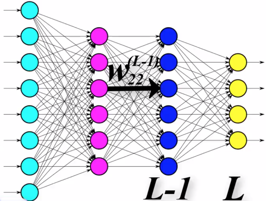
Suppose now we want to get the derivative of the error function with respect to a specific weight $w_{22}$: $$ \frac{\partial E}{\partial w_{22}} = \underbrace{\frac{\partial E}{\partial a_{2}^{(L-1)}}}_{\text{term 1}} \cdot \underbrace{\frac{\partial a_{2}^{(L-1)}}{\partial z_{2}^{(L-1)}}}_{\text{term 2}} \cdot \underbrace{\frac{\partial z_{2}^{(L-1)}}{\partial w_{22}^{(L-1)}}}_{\text{term 3}}, \tag{d} $$ which is very similar to equation $(b)$ which was used to calculate the derivative $\frac{\partial E}{\partial w_{12}^{(L)}}$.
Computing terms $2$ and $3$ are done exactly the same as for $\frac{\partial E}{\partial w_{12}^{(L)}}$. The problem is determining term $1$, since
Computing Term 1:
The term $\frac{\partial E}{\partial a_{2}^{(L-1)}}$ measures how much the error function changes when you make a small change to the activation of node $2$ in layer $L-1$. The value of this is $$ \begin{align} \frac{\partial E}{\partial a_{2}^{(L-1)}} &= \sum_{i=0}^{n-1} \Big( \frac{\partial E}{\partial a_j^{(L)}} \cdot \frac{\partial a_j^{(L)}}{\partial z_j^{(L)}} \cdot \frac{\partial z_j^{(L)}}{\partial a_2^{(L-1)}}\Big) \\ &= \sum_{i=0}^{n-1} \Big( (a_j^{(L)} - y_j) \cdot (g'^{(L)}) \cdot (w_{j2}^{(L)}) \Big) \end{align} $$
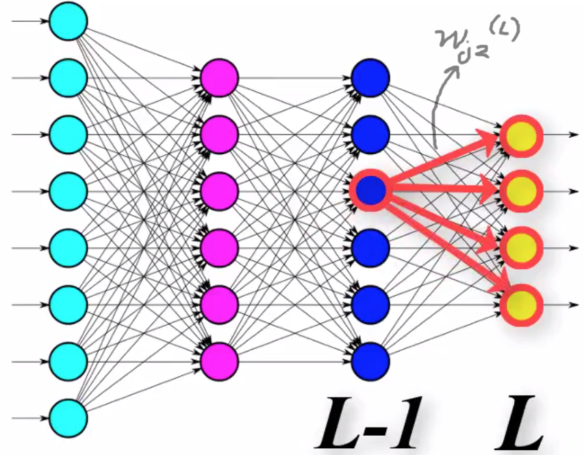
Now, the derivative $\frac{\partial E}{\partial w_{22}}$ is given as: $$ \begin{align} \frac{\partial E}{\partial w_{22}} &= \sum_{i=0}^{n-1} \Big( \underbrace{\frac{\partial E}{\partial a_j^{(L)}} \cdot \frac{\partial a_j^{(L)}}{\partial z_j^{(L)}}}_{\text{Passed back from the layer L}} \cdot \frac{\partial z_j^{(L)}}{\partial a_2^{(L-1)}}\Big) \cdot \underbrace{\frac{\partial a_{2}^{(L-1)}}{\partial z_{2}^{(L-1)}}}_{\text{term 2}} \cdot \underbrace{\frac{\partial z_{2}^{(L-1)}}{\partial w_{22}^{(L-1)}}}_{\text{term 3}} \\ &= \sum_{i=0}^{n-1} \Big( \underbrace{(a_j^{(L)} - y_j) \cdot (g'^{(L)})}_{\text{Passed back from the layer L}} \cdot (w_{j2}^{(L)}) \Big) \cdot \underbrace{\frac{\partial a_{2}^{(L-1)}}{\partial z_{2}^{(L-1)}}}_{\text{term 2}} \cdot \underbrace{\frac{\partial z_{2}^{(L-1)}}{\partial w_{22}^{(L-1)}}}_{\text{term 3}}, \tag{d} \end{align} $$
Calculating the derivative of the error with respect to any weight going towards node $j$ in any layer $l$ depends on the value $\frac{\partial E}{\partial a_j^{(l+1)}} \cdot \frac{\partial a_j^{(l+1)}}{\partial z_j^{(l+1)}}$ calculated from the layer in front.