Perceptrons
A perceptron models a biological neuron with an algorithm for the supervised learning of a binary classification of inputs. Put simply, a perceptron is just an algorithm for learning a threshold function — ie. a function that maps a vector $x$ to either $0$ or $1$, hence classifying that vector.
- The single-layer perceptron is the simplest example of a feed-forward artificial neural network. It is only capable of learning linearly-separable datapoints
McCulloch and Pitts Neuron (1943):
McCulloch and Pitts proposed the first computational model of a biological neuron in 1943. This precedes the invention of the perceptron algorithm in 1958.
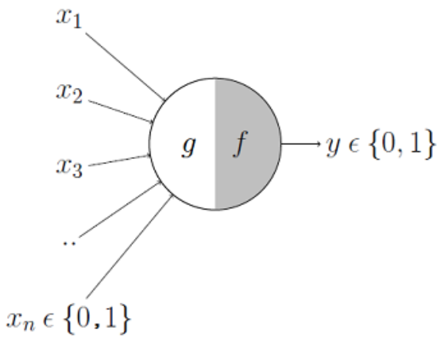
This is where it all began The left side of the neuron takes in inputs and computes an aggregated value, and the right side takes in that aggregated value and outputs a decision. The input vector models the electrochemical signals a biological neuron receives through its dendrites. > The function $g$ just directly sums the boolean inputs, plus a bias term. The function $f$ decides to output $0$ or $1$ based on whether $g(x)>\theta$, where $\theta$ is some threshold value. |
|
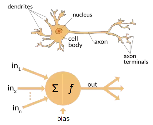
Rosenblatt's Perceptron (1958):
Rosenblatt's perceptron model extends the McCulloch-Pitts neuron model, except it takes in a vector of continuous real numbers and performs a weighted sum rather than a direct sum.
| Single-Layer Perceptron | Alternative Diagram |
|---|---|
 |
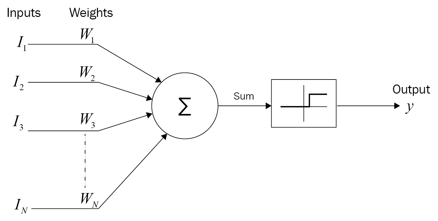 |
Activation function — translates the aggregated input signals to an output signal. Usually used interchangeably with the term 'transfer function'
Bias — a constant term that offsets the weighted sum, independent of the input. A positive bias means this neuron is more predisposed to firing
Perceptron Learning Algorithm:
The process of 'learning' in a single-layer perceptron model is the process of adjusting the weights until it can correctly map an input to the correct output class.
The perceptron makes a prediction by taking the dot product of the input vector and weight vector and adding the bias, then passing that through an activation function, for instance, the Heaviside step function:
$$g(s) = \begin{cases} 1, & s \geq 0,\\ 0, & s < 0. \tag{1} \end{cases}$$Perceptron Learning Rule:
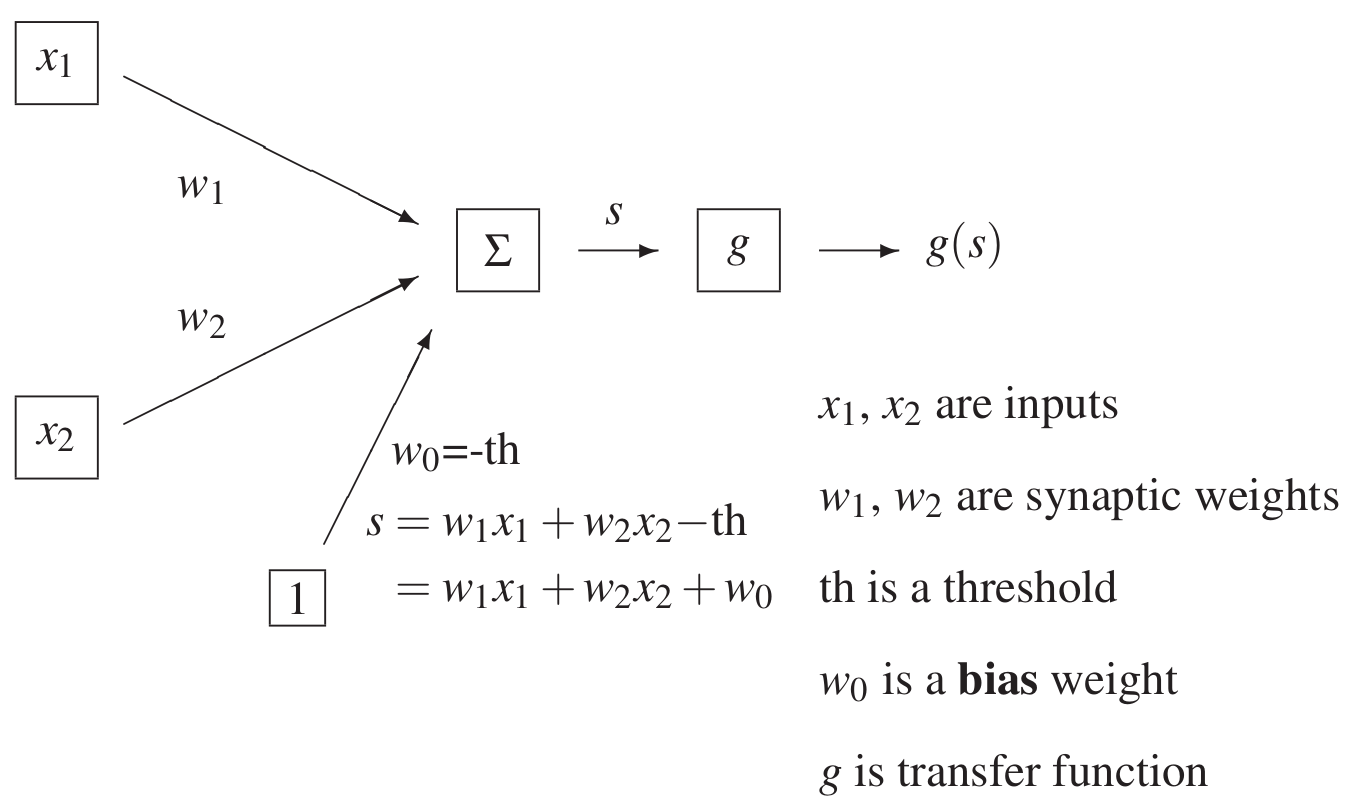
Suppose we have a perceptron that just takes in a vector with 2 components: $x=[x_1, x_2]$.
The perceptron takes in the input vector $x=[x_1, x_2]$ and has weights $w = [w_1, w_2]$ and an additional bias term $w_0$. Taking the dot product, we get $x \cdot w =w_1 x_1 + w_2 x_2$.
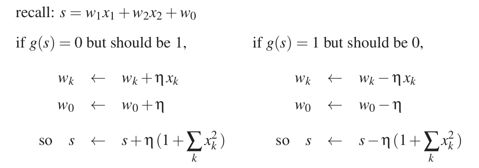
The aggregated sum is $s = w_1 x_1 + w_2 x_2 + w_0$. Once we pass this through the transfer function in $(1)$, $g(s)$, we get the predicted class that the input $x=[x_1, x_2]$ belongs to.
If the predicted class was incorrect, then we must adjust the weights of the perceptron, $w=[w_1, w_2]$ and $w_0$, so that future predictions will be more likely to correctly classify this input.
When we make updates to the weights, we use a factor term $\eta$, called the learning rate. This affects how much the weights of the perceptron are updated by. A large learning rate allows the
If $g(s)=0$ but the correct class was $1$, then we reassign the weights: $$
  \begin{align}
  w_0 &:= w_0 + \eta \\
  w_1 &:= w_1 + \eta x_1 \\
  w_2 &:= w_2 + \eta x_2.
  \end{align}
$$ Now, in the future when we receive the same input, the value $g(s)$ will be larger and therefore the perceptron will more likely output $g(s)=1$, the correct class.
If $g(s)=1$ but the correct class was $0$, then we reassign the weights: $$
  \begin{align}
  w_0 &:= w_0 - \eta \\
  w_1 &:= w_1 - \eta x_1 \\
  w_2 &:= w_2 - \eta x_2.
  \end{align}
$$ Now, in the future when we receive the same input, the value $g(s)$ will be lower and therefore the perceptron will more likely output $g(s)=0$, the correct class.
If the output class was correct, then no learning is done
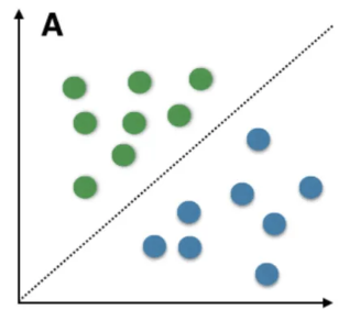
Linear Separability:
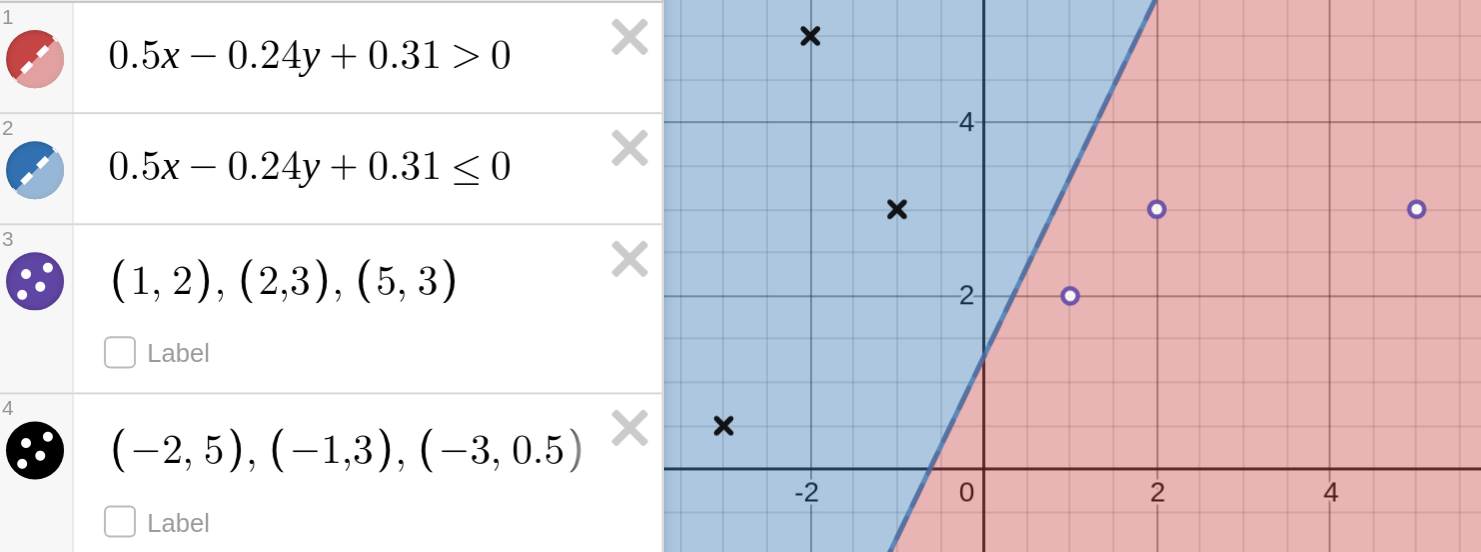
The weight vector of the perceptron model with $w=[w_1, w_2]$ and which takes in inputs $x=[x_1, x_2]$ defines a straight line decision boundary with equation: $w_1x_1 + w_2x_2+w_0=0$.
Eg. suppose you have a perceptron with weight vector $w=[0.5, -0.24]$ and bias $w_0=0.31$. This defines a decision boundary with the equation $0.5x-0.24y+0.31=0$.
Note: if we had higher dimensional input vectors and weight vectors of size $n$, then the equation $w_0+w_1x_1+\dots + w_nx_n=0$ defines a hyperplane surface instead.
Rosenblatt mathematically proved that the perceptron learning algorithm guarantees that a decision boundary will be eventually 'learned', provided that the dataset is linearly separable.
The perceptron learning algorithm unfortunately never learns the correct decision boundary if the learning set is not linearly separable. A dataset is not linearly separable if there exists no hyperplane that can classify all inputs into the correct class.
- The classic example of this is the XOR function. XOR can't be learned by a single-layer perceptron because it is not linearly separable:
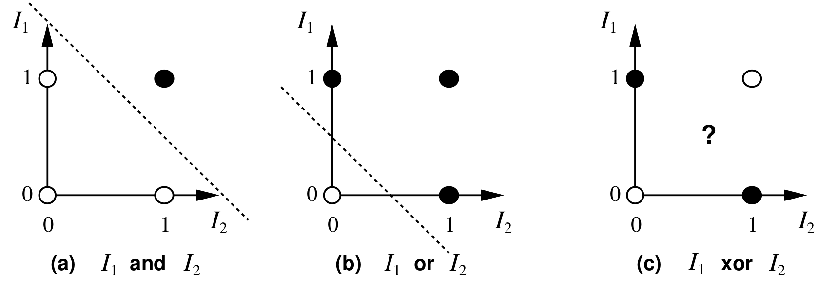 The XOR function can be learned by a multi-layer perceptron, however.
 - About multi-layer perceptrons:
- Multi-layer perceptrons can refer generally to any feedforward neural network, that is, any network where the connections between nodes don't form a cycle such that information 'flows' forward
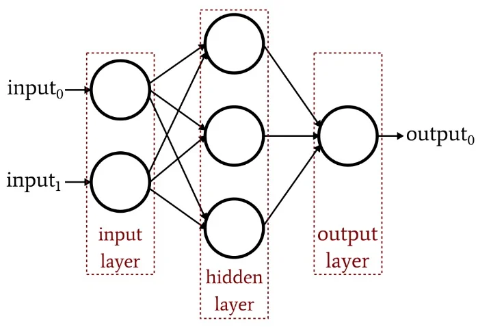
- With multi-layer perceptrons containing a hidden layer, we need a more sophisticated training method called backpropagation for updating the weights of the network
- Multi-layer perceptrons can refer generally to any feedforward neural network, that is, any network where the connections between nodes don't form a cycle such that information 'flows' forward